Chapter 16 附录2 表格可视化

McDonald, J. H. (2014). The Handbook of Biological Statistics (3rd ed.). SPARKY HOUSE PUBLISHING.

library(tidyverse)
library(languageR)
data("lexdec")

# show chinese characters in ggplot
library(showtext)
showtext_auto()

16.1 gt

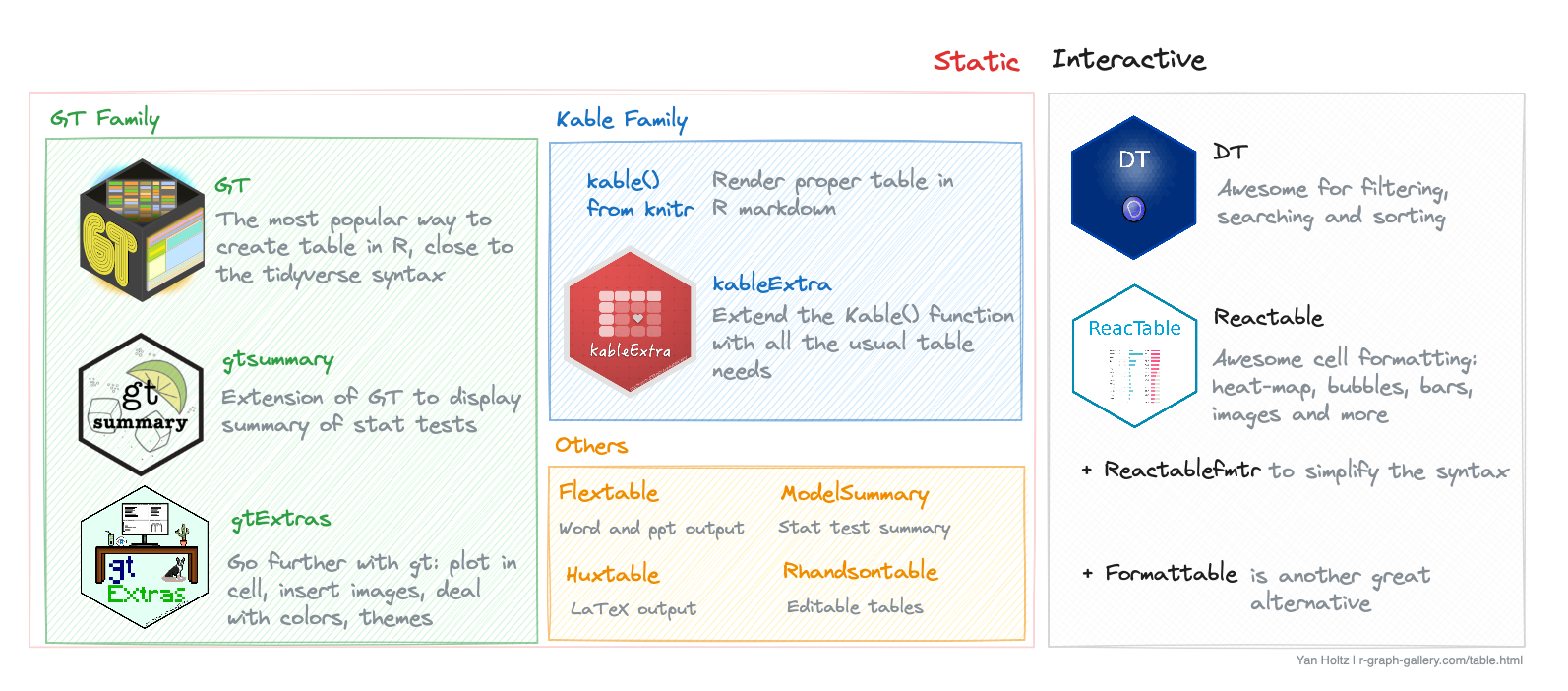
The gt package in R is a powerful tool for creating elegant and customizable tables for data visualization and reporting.

It offers options for formatting, styling, and theming tables, as well as support for handling complex data structures and creating publication-ready tables with ease.

The GT package, stands for “Grammar of Tables”. It was created by the RStudio team and first released in 2018. It offers an intuitive, tidyverse-inspired syntax, making table creation accessible, including for beginners.

GT’s user-friendly design for handling complex formatting has quickly gained popularity in the R community. Its ease of use and readability make it a go-to choice for many R users seeking to create clear and aesthetically pleasing tables.

library(gt)

lexdec%>% 
  group_by(Class, Correct, NativeLanguage)%>%
  summarise(mean = mean(RT))%>%
  ungroup()%>%
  gt()

## `summarise()` has grouped output by 'Class', 'Correct'. You can override using the `.groups`
## argument.

Class	Correct	NativeLanguage	mean
animal	correct	English	6.316985
animal	correct	Other	6.484137
animal	incorrect	English	6.210368
animal	incorrect	Other	6.542047
plant	correct	English	6.328352
plant	correct	Other	6.448381
plant	incorrect	English	6.162450
plant	incorrect	Other	6.631645

lexdec%>% 
  group_by(Class, Correct, NativeLanguage)%>%
  summarise(mean = mean(RT))%>%
  #ungroup()%>%
  gt()  

## `summarise()` has grouped output by 'Class', 'Correct'. You can override using the `.groups`
## argument.

NativeLanguage	mean
animal - correct
English	6.316985
Other	6.484137
animal - incorrect
English	6.210368
Other	6.542047
plant - correct
English	6.328352
Other	6.448381
plant - incorrect
English	6.162450
Other	6.631645

# 添加表格标题和副标题
lexdec%>% 
  group_by(Class, Correct, NativeLanguage)%>%
  summarise(mean = mean(RT))%>%
  ungroup()%>%
  gt() %>%
    tab_header(title = md("词汇**反应时**"),
               subtitle = md("不同词汇 *不同语言背景*"))

## `summarise()` has grouped output by 'Class', 'Correct'. You can override using the `.groups`
## argument.

词汇反应时
不同词汇 不同语言背景
Class	Correct	NativeLanguage	mean
animal	correct	English	6.316985
animal	correct	Other	6.484137
animal	incorrect	English	6.210368
animal	incorrect	Other	6.542047
plant	correct	English	6.328352
plant	correct	Other	6.448381
plant	incorrect	English	6.162450
plant	incorrect	Other	6.631645

# 添加脚注  
lexdec%>% 
  group_by(Class, Correct, NativeLanguage)%>%
  summarise(mean = mean(RT))%>%
  ungroup()%>%
  gt() %>%
  tab_footnote(
    footnote = "Source: lexdec package",
    locations = cells_body(columns = NativeLanguage, rows = 1)
  )

## `summarise()` has grouped output by 'Class', 'Correct'. You can override using the `.groups`
## argument.

Class	Correct	NativeLanguage	mean
animal	correct	English1	6.316985
animal	correct	Other	6.484137
animal	incorrect	English	6.210368
animal	incorrect	Other	6.542047
plant	correct	English	6.328352
plant	correct	Other	6.448381
plant	incorrect	English	6.162450
plant	incorrect	Other	6.631645
1 Source: lexdec package

lexdec%>% 
  group_by(Class, Correct, NativeLanguage)%>%
  summarise(mean = mean(RT))%>%
  ungroup()%>%
  gt() %>%
   tab_spanner(
    label = "词汇特征",
    columns = c(Class, Correct)) 

## `summarise()` has grouped output by 'Class', 'Correct'. You can override using the `.groups`
## argument.

词汇特征		NativeLanguage	mean
Class	Correct
animal	correct	English	6.316985
animal	correct	Other	6.484137
animal	incorrect	English	6.210368
animal	incorrect	Other	6.542047
plant	correct	English	6.328352
plant	correct	Other	6.448381
plant	incorrect	English	6.162450
plant	incorrect	Other	6.631645

16.1.1 gtsummary

The gtsummary package lets you automatically summarize information about your dataset. In the following case, we use the tbl_summary() function to obtain the main information on the iris dataset. The package detects the variable type and generates the appropriate summary type.

library(gtsummary)
lexdec%>% 
   tbl_summary()

Characteristic	N = 1,6591
Subject
A1	79 (4.8%)
A2	79 (4.8%)
A3	79 (4.8%)
C	79 (4.8%)
D	79 (4.8%)
I	79 (4.8%)
J	79 (4.8%)
K	79 (4.8%)
M1	79 (4.8%)
M2	79 (4.8%)
P	79 (4.8%)
R1	79 (4.8%)
R2	79 (4.8%)
R3	79 (4.8%)
S	79 (4.8%)
T1	79 (4.8%)
T2	79 (4.8%)
V	79 (4.8%)
W1	79 (4.8%)
W2	79 (4.8%)
Z	79 (4.8%)
RT	6.35 (6.21, 6.50)
Trial	106 (64, 146)
Sex
F	1,106 (67%)
M	553 (33%)
NativeLanguage
English	948 (57%)
Other	711 (43%)
Correct
correct	1,594 (96%)
incorrect	65 (3.9%)
PrevType
nonword	855 (52%)
word	804 (48%)
PrevCorrect
correct	1,542 (93%)
incorrect	117 (7.1%)
Word
almond	21 (1.3%)
ant	21 (1.3%)
apple	21 (1.3%)
apricot	21 (1.3%)
asparagus	21 (1.3%)
avocado	21 (1.3%)
banana	21 (1.3%)
bat	21 (1.3%)
beaver	21 (1.3%)
bee	21 (1.3%)
beetroot	21 (1.3%)
blackberry	21 (1.3%)
blueberry	21 (1.3%)
broccoli	21 (1.3%)
bunny	21 (1.3%)
butterfly	21 (1.3%)
camel	21 (1.3%)
carrot	21 (1.3%)
cat	21 (1.3%)
cherry	21 (1.3%)
chicken	21 (1.3%)
clove	21 (1.3%)
crocodile	21 (1.3%)
cucumber	21 (1.3%)
dog	21 (1.3%)
dolphin	21 (1.3%)
donkey	21 (1.3%)
eagle	21 (1.3%)
eggplant	21 (1.3%)
elephant	21 (1.3%)
fox	21 (1.3%)
frog	21 (1.3%)
gherkin	21 (1.3%)
goat	21 (1.3%)
goose	21 (1.3%)
grape	21 (1.3%)
gull	21 (1.3%)
hedgehog	21 (1.3%)
horse	21 (1.3%)
kiwi	21 (1.3%)
leek	21 (1.3%)
lemon	21 (1.3%)
lettuce	21 (1.3%)
lion	21 (1.3%)
magpie	21 (1.3%)
melon	21 (1.3%)
mole	21 (1.3%)
monkey	21 (1.3%)
moose	21 (1.3%)
mouse	21 (1.3%)
mushroom	21 (1.3%)
mustard	21 (1.3%)
olive	21 (1.3%)
orange	21 (1.3%)
owl	21 (1.3%)
paprika	21 (1.3%)
peanut	21 (1.3%)
pear	21 (1.3%)
pig	21 (1.3%)
pineapple	21 (1.3%)
potato	21 (1.3%)
radish	21 (1.3%)
reindeer	21 (1.3%)
shark	21 (1.3%)
sheep	21 (1.3%)
snake	21 (1.3%)
spider	21 (1.3%)
squid	21 (1.3%)
squirrel	21 (1.3%)
stork	21 (1.3%)
strawberry	21 (1.3%)
swan	21 (1.3%)
tomato	21 (1.3%)
tortoise	21 (1.3%)
vulture	21 (1.3%)
walnut	21 (1.3%)
wasp	21 (1.3%)
whale	21 (1.3%)
woodpecker	21 (1.3%)
Frequency	4.75 (3.95, 5.65)
FamilySize	0.00 (0.00, 1.10)
SynsetCount
0.6931472	189 (11%)
1.0986123	735 (44%)
1.3862944	273 (16%)
1.6094379	147 (8.9%)
1.7917595	84 (5.1%)
1.9459101	105 (6.3%)
2.0794415	63 (3.8%)
2.1972246	21 (1.3%)
2.3025851	42 (2.5%)
Length
3	168 (10%)
4	210 (13%)
5	399 (24%)
6	315 (19%)
7	189 (11%)
8	210 (13%)
9	105 (6.3%)
10	63 (3.8%)
Class
animal	924 (56%)
plant	735 (44%)
FreqSingular	69 (23, 146)
FreqPlural	49 (19, 132)
DerivEntropy	0.04 (0.00, 0.68)
Complex
complex	210 (13%)
simplex	1,449 (87%)
rInfl	0.19 (-0.30, 0.64)
meanRT	6.36 (6.32, 6.42)
SubjFreq	3.88 (3.16, 4.68)
meanSize	3.10 (1.89, 3.71)
meanWeight	2.76 (1.46, 3.42)
BNCw	3 (2, 7)
BNCc	1 (0, 3)
BNCd	4 (1, 10)
BNCcRatio	0.27 (0.10, 0.56)
BNCdRatio	0.93 (0.56, 2.13)
1 n (%); Median (IQR)

lexdec %>%
  select(Class, Correct, NativeLanguage, RT)%>%
  tbl_summary(
    by=NativeLanguage, # group by the `vs` variable (dichotomous: 0 or 1)
    statistic = list(
      all_continuous() ~ "{mean} ({sd})", # will display: mean (standard deviation)
      all_categorical() ~ "{n} / {N} ({p}%)" # will display: n / N (percentage)
    )
  ) %>%
  add_overall() %>% # statistics for all observations
  add_p() %>% # add p-values
  bold_labels() %>% # make label in bold
  italicize_levels() # make categories in label in italic

Characteristic	Overall, N = 1,6591	English, N = 9481	Other, N = 7111	p-value2
Class				>0.9
animal	924 / 1,659 (56%)	528 / 948 (56%)	396 / 711 (56%)
plant	735 / 1,659 (44%)	420 / 948 (44%)	315 / 711 (44%)
Correct				0.019
correct	1,594 / 1,659 (96%)	920 / 948 (97%)	674 / 711 (95%)
incorrect	65 / 1,659 (3.9%)	28 / 948 (3.0%)	37 / 711 (5.2%)
RT	6.39 (0.24)	6.32 (0.20)	6.47 (0.26)	<0.001
1 n / N (%); Mean (SD)
2 Pearson’s Chi-squared test; Wilcoxon rank sum test

16.1.2 gtExtras

gtExtras augments and expands the functionalities of the gt package. It allows to create even more sophisticated and visually appealing tables.

It comes with a set of themes to make your table good-looking with just one more line of code. It provides functions to easily add plots in table cells. It also has helper functions to help with colors and icons.

#install.packages("gtExtras")
library(gtExtras)

# create aggregated dataset
# agg_iris = iris %>%
#   group_by(Species) %>%
#   summarize(
#     Sepal.L = list(Sepal.Length),
#     Sepal.W = list(Sepal.Width),
#     Petal.L = list(Petal.Length),
#     Petal.W = list(Petal.Width)
#     )
library(languageR)
data(lexdec)

agg_lexdec = lexdec %>%
  select( NativeLanguage, RT, Frequency, FamilySize)%>%
  group_by(NativeLanguage)%>%
   summarize(
    RT= list(RT),
    Frequency = list(Frequency),
    FamilySize = list(FamilySize)
    )
# display the table with default output with gt package
agg_lexdec  %>%
  gt()



agg_lexdec %>%
  gt() %>%
  gt_plt_sparkline(RT) %>%
  gt_plt_sparkline(Frequency) %>%
  gt_plt_sparkline(FamilySize)


agg_lexdec %>%
  gt() %>%
  gt_plt_dist(
   RT,
    type = "density" 
  ) %>%
  gt_plt_dist( 
    Frequency,
    type = "boxplot"
  ) %>%
  gt_plt_dist( 
    FamilySize,
    type = "histogram"
  ) 

head(lexdec) %>%
  select( NativeLanguage, RT, Frequency, FamilySize)%>%
  gt() %>%
  gt_plt_bar_pct(
    RT,
    labels = TRUE
  ) %>%
  gt_plt_bar_pct(
    Frequency,
    labels=FALSE,
    fill = "forestgreen"
  )

lexdec%>%
  select( NativeLanguage, RT, Frequency, FamilySize)%>%
  gt_plt_summary()

16.2 DT: easy filtering & sorting

DT stands for “DataTables”, the Javascript library it interacts with. DT stands out for its ability to handle large datasets efficiently and its rich array of features like searching, sorting, and pagination.

I love adding a DT table at the beginning of my data analysis Quarto report. It provides access to your raw data easily!

Please check my full introduction to DT for more! Oh and this is how a DT table looks like:

library(DT)

lex.table <- 
  datatable(lexdec,
  filter = "top",
  class = 'cell-border stripe hover compact'
) # put it at the top of the table

flextable is another solid option to create very polish static tables. It supports a wide range of formatting options, including merging cells, rotating text, and conditional formatting.

It stands out due to its compatibility with various R Markdown formats, including Word, PowerPoint, and HTML.

library(flextable)
set_flextable_defaults(
  font.family = "Arial", font.size = 10, 
  border.color = "gray", big.mark = "")

ft <- flextable(head(lexdec)) |> 
  bold(part = "header") 
ft

Subject	RT	Trial	Sex	NativeLanguage	Correct	PrevType	PrevCorrect	Word	Frequency	FamilySize	SynsetCount	Length	Class	FreqSingular	FreqPlural	DerivEntropy	Complex	rInfl	meanRT	SubjFreq	meanSize	meanWeight	BNCw	BNCc	BNCd	BNCcRatio	BNCdRatio
A1	6.340359	23	F	English	correct	word	correct	owl	4.859812	1.3862944	0.6931472	3	animal	54	74	0.7912	simplex	-0.3101549	6.3582	3.12	3.4758	3.1806	12.057065	0.000000	6.175602	0.000000	0.512198
A1	6.308098	27	F	English	correct	nonword	correct	mole	4.605170	1.0986123	1.9459101	4	animal	69	30	0.6968	simplex	0.8145080	6.4150	2.40	2.9999	2.6112	5.738806	4.062251	2.850278	0.707856	0.496667
A1	6.349139	29	F	English	correct	nonword	correct	cherry	4.997212	0.6931472	1.6094379	6	plant	83	49	0.4754	simplex	0.5187938	6.3426	3.88	1.6278	1.2081	5.716520	3.249801	12.588727	0.568493	2.202166
A1	6.186209	30	F	English	correct	word	correct	pear	4.727388	0.0000000	1.0986123	4	plant	44	68	0.0000	simplex	-0.4274440	6.3353	4.52	1.9908	1.6114	2.050370	1.462410	7.363218	0.713242	3.591166
A1	6.025866	32	F	English	correct	nonword	correct	dog	7.667626	3.1354942	2.0794415	3	animal	1233	828	1.2129	simplex	0.3977961	6.2956	6.04	4.6429	4.5167	74.838494	50.859385	241.561040	0.679589	3.227765
A1	6.180017	33	F	English	correct	word	correct	blackberry	4.060443	0.6931472	1.3862944	10	plant	26	31	0.3492	complex	-0.1698990	6.3959	3.28	1.5831	1.1365	1.270338	0.162490	1.187616	0.127911	0.934882

ft |> 
  highlight(i = ~ RT > 6.3, j = "RT", color = "#ffe842") |> 
  bg(j = c("Frequency", "FamilySize", "Length"), 
     bg = scales::col_quantile(palette = c("wheat", "red"), domain =NULL)) |> 
  add_footer_lines("The 'lexdec' dataset")

## Warning: The following arguments are not supported:
## i, j
## Arguments such as: hoverinfo and showInLegend 
## have been replaced by selected and other

Subject	RT	Trial	Sex	NativeLanguage	Correct	PrevType	PrevCorrect	Word	Frequency	FamilySize	SynsetCount	Length	Class	FreqSingular	FreqPlural	DerivEntropy	Complex	rInfl	meanRT	SubjFreq	meanSize	meanWeight	BNCw	BNCc	BNCd	BNCcRatio	BNCdRatio
A1	6.340359	23	F	English	correct	word	correct	owl	4.859812	1.3862944	0.6931472	3	animal	54	74	0.7912	simplex	-0.3101549	6.3582	3.12	3.4758	3.1806	12.057065	0.000000	6.175602	0.000000	0.512198
A1	6.308098	27	F	English	correct	nonword	correct	mole	4.605170	1.0986123	1.9459101	4	animal	69	30	0.6968	simplex	0.8145080	6.4150	2.40	2.9999	2.6112	5.738806	4.062251	2.850278	0.707856	0.496667
A1	6.349139	29	F	English	correct	nonword	correct	cherry	4.997212	0.6931472	1.6094379	6	plant	83	49	0.4754	simplex	0.5187938	6.3426	3.88	1.6278	1.2081	5.716520	3.249801	12.588727	0.568493	2.202166
A1	6.186209	30	F	English	correct	word	correct	pear	4.727388	0.0000000	1.0986123	4	plant	44	68	0.0000	simplex	-0.4274440	6.3353	4.52	1.9908	1.6114	2.050370	1.462410	7.363218	0.713242	3.591166
A1	6.025866	32	F	English	correct	nonword	correct	dog	7.667626	3.1354942	2.0794415	3	animal	1233	828	1.2129	simplex	0.3977961	6.2956	6.04	4.6429	4.5167	74.838494	50.859385	241.561040	0.679589	3.227765
A1	6.180017	33	F	English	correct	word	correct	blackberry	4.060443	0.6931472	1.3862944	10	plant	26	31	0.3492	complex	-0.1698990	6.3959	3.28	1.5831	1.1365	1.270338	0.162490	1.187616	0.127911	0.934882
The 'lexdec' dataset

select(lexdec, c("Frequency", "FamilySize", 
                 "Length","NativeLanguage")) %>% 
  summarizor(by = c("NativeLanguage")) |> 
  flextable::as_flextable(spread_first_col = TRUE)

		English (N=948)		Other (N=711)
Frequency
Mean (SD)		4.8 (1.3)		4.8 (1.3)
Median (IQR)		4.8 (1.7)		4.8 (1.7)
Range		1.8 - 7.8		1.8 - 7.8
FamilySize
Mean (SD)		0.7 (0.9)		0.7 (0.9)
Median (IQR)		0.0 (1.1)		0.0 (1.1)
Range		0.0 - 3.3		0.0 - 3.3
Length
Mean (SD)		5.9 (1.9)		5.9 (1.9)
Median (IQR)		6.0 (2.0)		6.0 (2.0)
Range		3.0 - 10.0		3.0 - 10.0

16.3 modelsummary

library(modelsummary)
library(tinytable)
datasummary_skim(lexdec)

	Unique (#)	Missing (%)	Mean	SD	Min	Median	Max
RT	531	0	6.4	0.2	5.8	6.3	7.6
Trial	162	0	105.0	47.1	23.0	106.0	185.0
Frequency	74	0	4.8	1.3	1.8	4.8	7.8
FamilySize	13	0	0.7	0.9	0.0	0.0	3.3
SynsetCount	9	0	1.3	0.4	0.7	1.1	2.3
Length	8	0	5.9	1.9	3.0	6.0	10.0
FreqSingular	58	0	132.1	234.5	4.0	69.0	1518.0
FreqPlural	61	0	109.7	159.8	0.0	49.0	854.0
DerivEntropy	42	0	0.4	0.5	0.0	0.0	2.3
rInfl	72	0	0.3	0.9	−1.3	0.2	4.4
meanRT	79	0	6.4	0.1	6.2	6.4	6.6
SubjFreq	58	0	3.9	1.0	2.0	3.9	6.0
meanSize	78	0	2.9	1.0	1.3	3.1	4.8
meanWeight	78	0	2.6	1.0	0.8	2.8	4.7
BNCw	75	0	7.4	13.0	0.0	3.3	79.2
BNCc	35	0	5.0	13.6	0.0	0.6	83.2
BNCd	42	0	13.0	32.1	0.0	3.8	241.6
BNCcRatio	66	0	0.5	0.9	0.0	0.3	8.3
BNCdRatio	74	0	1.5	1.5	0.0	0.9	6.3

datasummary_balance(~NativeLanguage, lexdec)

## Warning: These variables were omitted because they include more than 50 levels: Word.

		English (N=948)		Other (N=711)
		Mean	Std. Dev.	Mean	Std. Dev.	Diff. in Means	Std. Error
RT		6.3	0.2	6.5	0.3	0.2	0.0
Trial		105.5	47.2	104.2	47.1	-1.3	2.3
Frequency		4.8	1.3	4.8	1.3	0.0	0.1
FamilySize		0.7	0.9	0.7	0.9	0.0	0.0
SynsetCount		1.3	0.4	1.3	0.4	0.0	0.0
Length		5.9	1.9	5.9	1.9	0.0	0.1
FreqSingular		132.1	234.5	132.1	234.6	0.0	11.6
FreqPlural		109.7	159.8	109.7	159.8	0.0	7.9
DerivEntropy		0.4	0.5	0.4	0.5	0.0	0.0
rInfl		0.3	0.9	0.3	0.9	0.0	0.0
meanRT		6.4	0.1	6.4	0.1	0.0	0.0
SubjFreq		3.9	1.0	3.9	1.0	0.0	0.1
meanSize		2.9	1.0	2.9	1.0	0.0	0.0
meanWeight		2.6	1.0	2.6	1.0	0.0	0.1
BNCw		7.4	13.0	7.4	13.0	0.0	0.6
BNCc		5.0	13.6	5.0	13.6	0.0	0.7
BNCd		13.0	32.1	13.0	32.1	0.0	1.6
BNCcRatio		0.5	0.9	0.5	0.9	0.0	0.0
BNCdRatio		1.5	1.5	1.5	1.5	0.0	0.1
		N	Pct.	N	Pct.
Subject	A1	79	8.3	0	0.0
	A2	79	8.3	0	0.0
	A3	0	0.0	79	11.1
	C	79	8.3	0	0.0
	D	0	0.0	79	11.1
	I	0	0.0	79	11.1
	J	0	0.0	79	11.1
	K	79	8.3	0	0.0
	M1	79	8.3	0	0.0
	M2	0	0.0	79	11.1
	P	0	0.0	79	11.1
	R1	79	8.3	0	0.0
	R2	79	8.3	0	0.0
	R3	79	8.3	0	0.0
	S	79	8.3	0	0.0
	T1	79	8.3	0	0.0
	T2	0	0.0	79	11.1
	V	0	0.0	79	11.1
	W1	79	8.3	0	0.0
	W2	79	8.3	0	0.0
	Z	0	0.0	79	11.1
Sex	F	553	58.3	553	77.8
	M	395	41.7	158	22.2
Correct	correct	920	97.0	674	94.8
	incorrect	28	3.0	37	5.2
PrevType	nonword	482	50.8	373	52.5
	word	466	49.2	338	47.5
PrevCorrect	correct	911	96.1	631	88.7
	incorrect	37	3.9	80	11.3
Class	animal	528	55.7	396	55.7
	plant	420	44.3	315	44.3
Complex	complex	120	12.7	90	12.7
	simplex	828	87.3	621	87.3

datasummary_correlation(lexdec)

	RT	Trial	Frequency	FamilySize	SynsetCount	Length	FreqSingular	FreqPlural	DerivEntropy	rInfl	meanRT	SubjFreq	meanSize	meanWeight	BNCw	BNCc	BNCd	BNCcRatio	BNCdRatio
RT	1	.	.	.	.	.	.	.	.	.	.	.	.	.	.	.	.	.	.
Trial	−.06	1	.	.	.	.	.	.	.	.	.	.	.	.	.	.	.	.	.
Frequency	−.23	.00	1	.	.	.	.	.	.	.	.	.	.	.	.	.	.	.	.
FamilySize	−.19	.02	.71	1	.	.	.	.	.	.	.	.	.	.	.	.	.	.	.
SynsetCount	−.18	.00	.49	.55	1	.	.	.	.	.	.	.	.	.	.	.	.	.	.
Length	.16	.01	−.43	−.63	−.33	1	.	.	.	.	.	.	.	.	.	.	.	.	.
FreqSingular	−.14	.02	.68	.67	.50	−.30	1	.	.	.	.	.	.	.	.	.	.	.	.
FreqPlural	−.16	.02	.76	.70	.39	−.36	.89	1	.	.	.	.	.	.	.	.	.	.	.
DerivEntropy	−.15	.00	.52	.85	.48	−.57	.37	.41	1	.	.	.	.	.	.	.	.	.	.
rInfl	.02	−.02	−.18	−.15	.16	.19	.06	−.21	−.14	1	.	.	.	.	.	.	.	.	.
meanRT	.34	.00	−.63	−.53	−.48	.45	−.39	−.45	−.42	.09	1	.	.	.	.	.	.	.	.
SubjFreq	−.23	.02	.50	.25	.31	−.08	.44	.45	.08	.05	−.63	1	.	.	.	.	.	.	.
meanSize	.00	−.02	.42	.36	−.05	−.24	.44	.50	.12	−.19	.00	−.21	1	.	.	.	.	.	.
meanWeight	−.01	−.02	.44	.37	−.04	−.25	.46	.52	.12	−.19	−.02	−.18	1.00	1	.	.	.	.	.
BNCw	−.13	.02	.64	.69	.45	−.32	.96	.87	.41	.03	−.37	.44	.42	.44	1	.	.	.	.
BNCc	−.09	.01	.48	.58	.41	−.30	.69	.64	.42	.03	−.25	.24	.31	.33	.72	1	.	.	.
BNCd	−.12	.01	.52	.49	.40	−.23	.79	.70	.24	.06	−.34	.53	.30	.32	.80	.49	1	.	.
BNCcRatio	−.03	−.01	.19	.23	.22	−.18	.12	.13	.24	.05	−.07	.01	.10	.10	.13	.74	.05	1	.
BNCdRatio	−.11	.01	.12	−.11	.10	.12	.13	.09	−.19	.10	−.32	.61	−.16	−.15	.09	−.02	.38	−.03	1

mod <- lm(RT ~ NativeLanguage, data = lexdec)

modelsummary(mod, output = "table.docx")

modelsummary(mod)

	Model 1
(Intercept)	6.318
	(0.007)
NativeLanguageOther	0.156
	(0.011)
Num.Obs.	1659
R2	0.102
R2 Adj.	0.101
AIC	−179.8
BIC	−163.6
Log.Lik.	92.917
F	188.227
RMSE	0.23